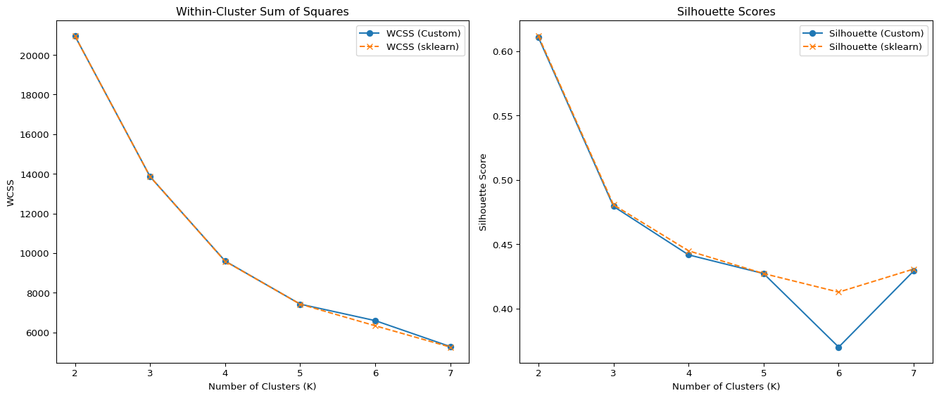
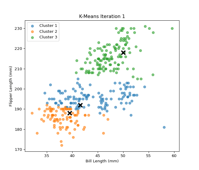
In this section, I implemented the K-Means clustering algorithm from scratch and tested it on the Palmer Penguins dataset using two numerical features: bill_length_mm and flipper_length_mm. The custom implementation includes steps for centroid initialization, cluster assignment, centroid updating, and calculation of within-cluster sum of squares (WCSS). I then evaluated clustering performance across different values of K (from 2 to 7) using both WCSS and silhouette scores. To validate the custom implementation, I compared the results with the built-in KMeans function from scikit-learn. The results show that both implementations behave similarly, and visualizations of WCSS and silhouette scores help identify the optimal number of clusters. This analysis provides insights into how well the data naturally groups into clusters and reinforces the value of silhouette and WCSS as clustering evaluation metrics.
import pandas as pdpenguins_df = pd.read_csv("palmer_penguins.csv")# Clean and filter the dataset: keep only bill_length_mm and flipper_length_mm, drop missing valuespenguins_filtered = penguins_df[['bill_length_mm', 'flipper_length_mm']].dropna()penguins_filtered.head()
bill_length_mm
flipper_length_mm
0
39.1
181
1
39.5
186
2
40.3
195
3
36.7
193
4
39.3
190
X_penguins = penguins_filtered.values
import numpy as npimport matplotlib.pyplot as plt# Custom K-Means implementationdef initialize_centroids(X, k): indices = np.random.choice(len(X), k, replace=False)return X[indices]def assign_clusters(X, centroids): distances = np.linalg.norm(X[:, np.newaxis] - centroids, axis=2)return np.argmin(distances, axis=1)def update_centroids(X, labels, k):return np.array([X[labels == i].mean(axis=0) for i inrange(k)])def compute_wcss(X, labels, centroids):returnsum(np.sum((X[labels == i] - centroids[i]) **2) for i inrange(len(centroids)))# Run K-Means from scratch for K = 2 to 7from sklearn.metrics import silhouette_scorefrom sklearn.cluster import KMeanswcss_vals = []silhouette_vals = []K_range =range(2, 8)for k in K_range: centroids = initialize_centroids(X_penguins, k)for _ inrange(10): labels = assign_clusters(X_penguins, centroids) centroids = update_centroids(X_penguins, labels, k) wcss = compute_wcss(X_penguins, labels, centroids) wcss_vals.append(wcss)iflen(np.unique(labels)) >1: silhouette = silhouette_score(X_penguins, labels) silhouette_vals.append(silhouette)else: silhouette_vals.append(np.nan)# Also compute sklearn KMeans for comparisonkmeans_models = [KMeans(n_clusters=k, n_init=10, random_state=0).fit(X_penguins) for k in K_range]wcss_sklearn = [model.inertia_ for model in kmeans_models]silhouette_sklearn = [silhouette_score(X_penguins, model.labels_) for model in kmeans_models]print("K-Means")print("K\tWCSS (Custom)\tSilhouette (Custom)")for i, k inenumerate(K_range): silhouette =f"{silhouette_vals[i]:.3f}"ifnot np.isnan(silhouette_vals[i]) else"NaN"print(f"{k}\t{wcss_vals[i]:.2f}\t\t{silhouette}")print("\nK\tWCSS (sklearn)\tSilhouette (sklearn)")for i, k inenumerate(K_range):print(f"{k}\t{wcss_sklearn[i]:.2f}\t\t{silhouette_sklearn[i]:.3f}")plt.figure(figsize=(14, 6))plt.subplot(1, 2, 1)plt.plot(K_range, wcss_vals, marker='o', label="WCSS (Custom)")plt.plot(K_range, wcss_sklearn, marker='x', linestyle='--', label="WCSS (sklearn)")plt.xlabel("Number of Clusters (K)")plt.ylabel("WCSS")plt.title("Within-Cluster Sum of Squares")plt.legend()plt.subplot(1, 2, 2)plt.plot(K_range, silhouette_vals, marker='o', label="Silhouette (Custom)")plt.plot(K_range, silhouette_sklearn, marker='x', linestyle='--', label="Silhouette (sklearn)")plt.xlabel("Number of Clusters (K)")plt.ylabel("Silhouette Score")plt.title("Silhouette Scores")plt.legend()plt.tight_layout()plt.show()
Based on the evaluation of both within-cluster sum of squares (WCSS) and silhouette scores for values of K ranging from 2 to 7, the optimal number of clusters appears to be K = 3. While the silhouette score is highest at K = 2, suggesting strong cohesion and separation, this may overly simplify the data into just two broad groups. K = 3 provides a more detailed segmentation while still maintaining a relatively high silhouette score and a substantial drop in WCSS, indicating a good trade-off between compactness and separation of clusters. Thus, K = 3 is suggested as the most appropriate choice by these two metrics.
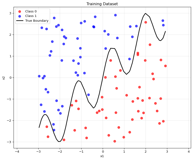
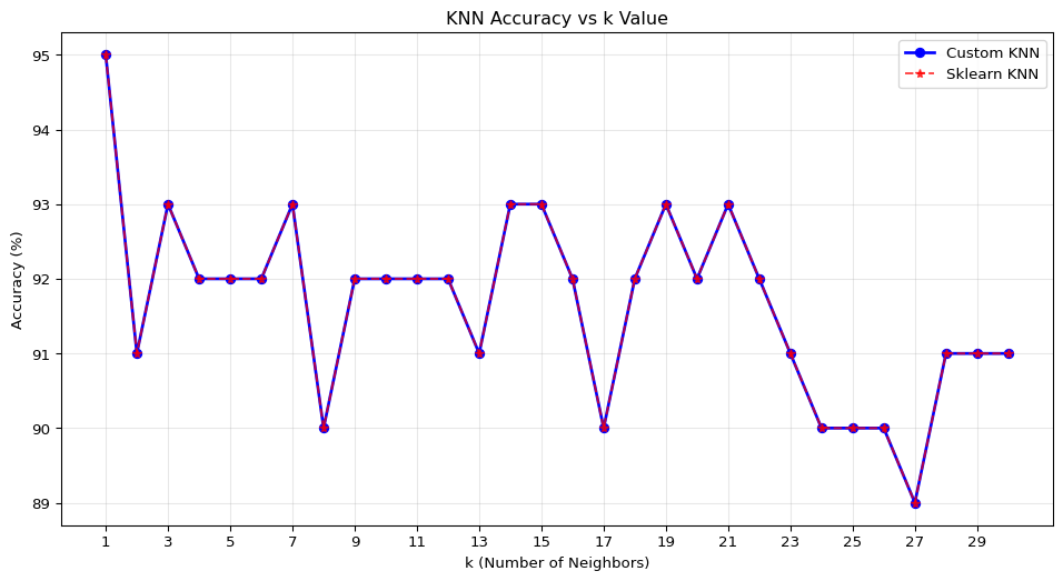
To evaluate the k-nearest neighbors (KNN) algorithm, I generated a synthetic dataset with two features (x1, x2) and a binary outcome y, where the class label is determined by whether x2 lies above or below a wiggly boundary defined by sin(4x1) + x1. The training dataset was visualized with points colored by class and the true decision boundary clearly drawn. A separate test dataset of 100 points was created using a different random seed to ensure independence. I implemented KNN from scratch and verified its correctness by comparing predictions with those from scikit-learn’s KNeighborsClassifier. The results were identical across all k values. I evaluated model performance for k = 1 to 30, recording the percentage of correctly classified test points. Accuracy was plotted against k, and the optimal value was found to be k = 1, achieving a 95% test accuracy. This highlights how a low k can capture fine-grained decision boundaries in data with nonlinear separability.
import numpy as npimport matplotlib.pyplot as pltfrom sklearn.neighbors import KNeighborsClassifierfrom sklearn.metrics import accuracy_scoreimport pandas as pdnp.random.seed(42)def generate_dataset(n=100, seed=42):"""Generate synthetic dataset with wiggly boundary""" np.random.seed(seed)# Generate random points x1 = np.random.uniform(-3, 3, n) x2 = np.random.uniform(-3, 3, n)# Define wiggly boundary boundary = np.sin(4* x1) + x1# Binary classification based on boundary y = (x2 > boundary).astype(int)return x1, x2, y, boundarydef plot_dataset(x1, x2, y, boundary=None, title="Dataset"):"""Plot the dataset with optional boundary""" plt.figure(figsize=(10, 8))# Plot points colored by class colors = ['red', 'blue'] labels = ['Class 0', 'Class 1']for i in [0, 1]: mask = y == i plt.scatter(x1[mask], x2[mask], c=colors[i], label=labels[i], alpha=0.7, s=50)if boundary isnotNone:# Sort by x1 for smooth boundary line sorted_idx = np.argsort(x1) plt.plot(x1[sorted_idx], boundary[sorted_idx], 'black', linewidth=2, label='True Boundary') plt.xlabel('x1') plt.ylabel('x2') plt.title(title) plt.legend() plt.grid(True, alpha=0.3) plt.axis('equal') plt.show()def euclidean_distance(point1, point2):"""Calculate Euclidean distance between two points"""return np.sqrt(np.sum((point1 - point2) **2))def knn_predict(X_train, y_train, X_test, k):""" Hand-implemented KNN classifier Parameters: X_train: Training features (n_samples, n_features) y_train: Training labels (n_samples,) X_test: Test features (m_samples, n_features) k: Number of neighbors Returns: predictions: Predicted labels for test set """ predictions = []for test_point in X_test:# Calculate distances to all training points distances = []for i, train_point inenumerate(X_train): dist = euclidean_distance(test_point, train_point) distances.append((dist, y_train[i]))# Sort by distance and get k nearest neighbors distances.sort(key=lambda x: x[0]) k_nearest = distances[:k]# Get labels of k nearest neighbors neighbor_labels = [label for _, label in k_nearest]# Predict based on majority vote prediction =max(set(neighbor_labels), key=neighbor_labels.count) predictions.append(prediction)return np.array(predictions)# Generate training datasetprint("Generating training dataset...")x1_train, x2_train, y_train, boundary_train = generate_dataset(n=100, seed=42)X_train = np.column_stack((x1_train, x2_train))# Plot training datasetplot_dataset(x1_train, x2_train, y_train, boundary_train, "Training Dataset")# Generate test dataset with different seedprint("Generating test dataset...")x1_test, x2_test, y_test, boundary_test = generate_dataset(n=100, seed=123)X_test = np.column_stack((x1_test, x2_test))# Test KNN implementation for different k valuesk_values =range(1, 31)accuracies_custom = []accuracies_sklearn = []print("Testing KNN for k = 1 to 30...")for k in k_values:# Custom KNN implementation y_pred_custom = knn_predict(X_train, y_train, X_test, k) accuracy_custom = accuracy_score(y_test, y_pred_custom) accuracies_custom.append(accuracy_custom)# Sklearn KNN for comparison knn_sklearn = KNeighborsClassifier(n_neighbors=k) knn_sklearn.fit(X_train, y_train) y_pred_sklearn = knn_sklearn.predict(X_test) accuracy_sklearn = accuracy_score(y_test, y_pred_sklearn) accuracies_sklearn.append(accuracy_sklearn)print(f"k={k:2d}: Custom KNN = {accuracy_custom:.3f}, Sklearn KNN = {accuracy_sklearn:.3f}")# Verify implementations matchprint(f"\nImplementations match: {np.allclose(accuracies_custom, accuracies_sklearn)}")# Plot accuracy vs kplt.figure(figsize=(12, 6))plt.plot(k_values, [acc *100for acc in accuracies_custom], 'bo-', label='Custom KNN', linewidth=2)plt.plot(k_values, [acc *100for acc in accuracies_sklearn], 'r*--', label='Sklearn KNN', alpha=0.7)plt.xlabel('k (Number of Neighbors)')plt.ylabel('Accuracy (%)')plt.title('KNN Accuracy vs k Value')plt.legend()plt.grid(True, alpha=0.3)plt.xticks(range(1, 31, 2))plt.show()# Find optimal koptimal_k = k_values[np.argmax(accuracies_custom)]max_accuracy =max(accuracies_custom)print(f"\nOptimal k value: {optimal_k}")print(f"Maximum accuracy: {max_accuracy:.3f} ({max_accuracy*100:.1f}%)")# Create summary tableresults_df = pd.DataFrame({'k': k_values,'Custom_KNN_Accuracy': [f"{acc:.3f}"for acc in accuracies_custom],'Sklearn_KNN_Accuracy': [f"{acc:.3f}"for acc in accuracies_sklearn]})print(f"\nSummary of first 10 k values:")print(results_df.head(10).to_string(index=False))