This assignment expores two methods for estimating the MNL model: (1) via Maximum Likelihood, and (2) via a Bayesian approach using a Metropolis-Hastings MCMC algorithm.
1. Likelihood for the Multi-nomial Logit (MNL) Model
Suppose we have \(i=1,\ldots,n\) consumers who each select exactly one product \(j\) from a set of \(J\) products. The outcome variable is the identity of the product chosen \(y_i \in \{1, \ldots, J\}\) or equivalently a vector of \(J-1\) zeros and \(1\) one, where the \(1\) indicates the selected product. For example, if the third product was chosen out of 3 products, then either \(y=3\) or \(y=(0,0,1)\) depending on how we want to represent it. Suppose also that we have a vector of data on each product \(x_j\) (eg, brand, price, etc.).
We model the consumer’s decision as the selection of the product that provides the most utility, and we’ll specify the utility function as a linear function of the product characteristics:
\[ U_{ij} = x_j'\beta + \epsilon_{ij} \]
where \(\epsilon_{ij}\) is an i.i.d. extreme value error term.
The choice of the i.i.d. extreme value error term leads to a closed-form expression for the probability that consumer \(i\) chooses product \(j\):
A clever way to write the individual likelihood function for consumer \(i\) is the product of the \(J\) probabilities, each raised to the power of an indicator variable (\(\delta_{ij}\)) that indicates the chosen product:
We will simulate data from a conjoint experiment about video content streaming services. We elect to simulate 100 respondents, each completing 10 choice tasks, where they choose from three alternatives per task. For simplicity, there is not a “no choice” option; each simulated respondent must select one of the 3 alternatives.
Each alternative is a hypothetical streaming offer consistent of three attributes: (1) brand is either Netflix, Amazon Prime, or Hulu; (2) ads can either be part of the experience, or it can be ad-free, and (3) price per month ranges from $4 to $32 in increments of $4.
The part-worths (ie, preference weights or beta parameters) for the attribute levels will be 1.0 for Netflix, 0.5 for Amazon Prime (with 0 for Hulu as the reference brand); -0.8 for included adverstisements (0 for ad-free); and -0.1*price so that utility to consumer \(i\) for hypothethical streaming service \(j\) is
where the variables are binary indicators and \(\varepsilon\) is Type 1 Extreme Value (ie, Gumble) distributed.
The following code provides the simulation of the conjoint data.
Note
import numpy as npimport pandas as pd# Set seed for reproducibilitynp.random.seed(123)# Define attributesbrands = ["N", "P", "H"] # Netflix, Prime, Huluads = ["Yes", "No"]prices = np.arange(8, 33, 4) # From 8 to 32 inclusive, step 4# Generate all possible profilesprofiles = pd.DataFrame( [(b, a, p) for b in brands for a in ads for p in prices], columns=["brand", "ad", "price"])m =len(profiles)# Assign part-worth utilities (true parameters)b_util = {"N": 1.0, "P": 0.5, "H": 0.0}a_util = {"Yes": -0.8, "No": 0.0}p_util =lambda p: -0.1* p# Parameters for the simulationn_peeps =100n_tasks =10n_alts =3# Function to simulate one respondent's datadef simulate_one_respondent(resp_id): records = []for t inrange(1, n_tasks +1):# Sample 3 random alternatives sampled = profiles.sample(n=n_alts).copy() sampled["resp"] = resp_id sampled["task"] = t# Compute deterministic utility sampled["v"] = ( sampled["brand"].map(b_util) + sampled["ad"].map(a_util) + sampled["price"].apply(p_util) )# Add Gumbel noise (Type I extreme value) sampled["e"] =-np.log(-np.log(np.random.rand(n_alts))) sampled["u"] = sampled["v"] + sampled["e"]# Identify chosen alternative (1 = chosen, 0 = not) sampled["choice"] = (sampled["u"] == sampled["u"].max()).astype(int) records.append(sampled[["resp", "task", "brand", "ad", "price", "choice"]])return pd.concat(records, ignore_index=True)# Simulate data for all respondentsconjoint_data = pd.concat( [simulate_one_respondent(i) for i inrange(1, n_peeps +1)], ignore_index=True)# Display first few rowsconjoint_data.head()
resp
task
brand
ad
price
choice
0
1
1
P
No
32
0
1
1
1
N
No
28
0
2
1
1
N
No
24
1
3
1
2
H
No
28
0
4
1
2
H
No
8
1
3. Preparing the Data for Estimation
The “hard part” of the MNL likelihood function is organizing the data, as we need to keep track of 3 dimensions (consumer \(i\), covariate \(k\), and product \(j\)) instead of the typical 2 dimensions for cross-sectional regression models (consumer \(i\) and covariate \(k\)). The fact that each task for each respondent has the same number of alternatives (3) helps. In addition, we need to convert the categorical variables for brand and ads into binary variables.
import pandas as pdconjoint_data = pd.read_csv("conjoint_data.csv")conjoint_data.head()
The dataset contains 3,000 observations from a choice based conjoint survey. Each respondent completed several tasks, each involving three product alternatives, and selected one option per task. There are 1,000 unique tasks, suggesting about 333 respondents each completed three tasks.
The dataset includes both categorical and numerical variables. The categorical variables include brand (H, N, P) and ad (Yes or No), which were converted to binary indicators using one hot encoding, with one category dropped to avoid multicollinearity. Price is a numerical variable. The response variable, choice, indicates the selected product in each task, with exactly one choice per task.
4. Estimation via Maximum Likelihood
import numpy as npfrom scipy.optimize import minimizefrom numpy.linalg import invdef negative_log_likelihood(beta, X, y, choice_ids): Xb = X @ beta Xb = np.asarray(Xb, dtype=np.float64) df = pd.DataFrame({"Xb": Xb,"y": y,"choice_id": choice_ids })# Compute softmax denominators per choice set df["exp_Xb"] = np.exp(df["Xb"]) denom = df.groupby("choice_id")["exp_Xb"].transform("sum") df["prob"] = df["exp_Xb"] / denom# Log likelihood contribution only from chosen alternatives log_likelihood = np.sum(df["y"] * np.log(df["prob"]))return-log_likelihood # negate because we minimize
# Inverse Hessian = estimated variance-covariance matrixhess_inv = result.hess_invse = np.sqrt(np.diag(hess_inv)) # Standard errors# 95% Confidence intervalsz =1.96conf_int = np.column_stack((beta_hat - z * se, beta_hat + z * se))param_names = X.columns.tolist()summary_df = pd.DataFrame({"Parameter": param_names,"Estimate": beta_hat,"Std. Error": se,"95% CI Lower": conf_int[:, 0],"95% CI Upper": conf_int[:, 1]})summary_df
Parameter
Estimate
Std. Error
95% CI Lower
95% CI Upper
0
brand_N
0.941195
0.105751
0.733922
1.148468
1
brand_P
0.501616
0.101876
0.301939
0.701292
2
ad_Yes
-0.731994
0.088966
-0.906369
-0.557620
3
price
-0.099480
0.006366
-0.111958
-0.087003
The maximum likelihood estimation results provide insights into consumer preferences based on the estimated coefficients. The coefficient for brand_N is the highest at 0.94, indicating a strong positive preference relative to the baseline brand. Brand_P also has a positive effect (0.50), though smaller. The presence of ads has a significant negative impact on choice, with a coefficient of -0.73. Price is also negatively associated with choice, as expected, with a coefficient of -0.10. All estimates are statistically significant, with 95% confidence intervals that do not cross zero, confirming the reliability of the effects.
5. Estimation via Bayesian Methods
import numpy as npimport pandas as pdfrom sklearn.preprocessing import LabelEncoder# Assume df is your already-preprocessed dataframeX = df[["brand_N", "brand_P", "ad_Yes", "price"]].astype(np.float64).values# Encode choice setsgroup_ids = LabelEncoder().fit_transform(choice_ids)num_sets = group_ids.max() +1# Build group mapping matrix (num_sets x num_observations)group_matrix = np.zeros((num_sets, X.shape[0]))group_matrix[group_ids, np.arange(X.shape[0])] =1# Vectorized log-likelihooddef negative_log_likelihood(beta, X, y, group_ids, group_matrix): beta = np.asarray(beta, dtype=np.float64) utilities = X @ beta exp_utilities = np.exp(utilities) denom = group_matrix @ exp_utilities probabilities = exp_utilities / denom[group_ids] log_likelihood = np.sum(np.log(probabilities[y ==1] +1e-12)) # Add epsilon for safetyreturn-log_likelihood # Return negative log-likelihood# Log-prior with N(0,5) for first 3, N(0,1) for pricedef log_prior(beta): beta = np.asarray(beta) prior_sd = np.array([5.0, 5.0, 5.0, 1.0])return-0.5* np.sum((beta / prior_sd) **2)# Log-posteriordef log_posterior(beta):return-negative_log_likelihood(beta, X, y, group_ids, group_matrix) + log_prior(beta)# Proposal standard deviationsproposal_sd = np.array([0.05, 0.05, 0.05, 0.005])def metropolis_hastings(log_posterior, start, iterations=11000, burn=1000): beta_current = np.asarray(start) samples = [] accepted =0for i inrange(iterations): proposal = beta_current + np.random.normal(0, proposal_sd) log_alpha = log_posterior(proposal) - log_posterior(beta_current)if np.log(np.random.rand()) < log_alpha: beta_current = proposal accepted +=1if i >= burn: samples.append(beta_current.copy())print(f"Acceptance rate: {accepted / iterations:.3f}")return np.array(samples)np.random.seed(42)posterior_samples = metropolis_hastings(log_posterior, start=np.zeros(4))
Acceptance rate: 0.567
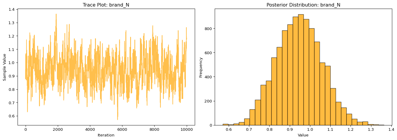
import matplotlib.pyplot as plt# Choose the parameter index for brand_Nbeta_index =0param_label ="brand_N"samples = posterior_samples[:, beta_index]# Create plotsplt.figure(figsize=(14, 5))# Trace plotplt.subplot(1, 2, 1)plt.plot(samples, alpha=0.7, color='orange')plt.title(f"Trace Plot: {param_label}")plt.xlabel("Iteration")plt.ylabel("Sample Value")# Histogramplt.subplot(1, 2, 2)plt.hist(samples, bins=30, edgecolor='k', alpha=0.75, color='orange')plt.title(f"Posterior Distribution: {param_label}")plt.xlabel("Value")plt.ylabel("Frequency")plt.tight_layout()plt.show()
The trace plot for the brand_N parameter shows good mixing and stability across iterations, indicating that the MCMC sampler has converged and is effectively exploring the posterior distribution. There are no visible trends or autocorrelation patterns, which supports the reliability of the sampling process. The histogram of the posterior distribution is approximately bell-shaped and centered around 0.95, suggesting a strong and consistent positive effect of the brand_N attribute on choice probability across sampled draws. This reinforces the conclusion that respondents significantly prefer brand N over the baseline brand.
The summary of the posterior estimates reveals clear consumer preferences among the product attributes. Both brand_N and brand_P have positive and statistically significant effects, with brand_N showing a stronger impact, indicating a higher preference for this brand over the baseline. The coefficient for ad_Yes is negative, suggesting that advertising is generally disliked by respondents. As expected, the price coefficient is also negative and precisely estimated, confirming that higher prices reduce the likelihood of a product being chosen. All parameters have narrow 95% credible intervals that do not include zero, reinforcing the strength and significance of these effects.
6. Discussion
If the data had not been simulated and instead came from a real conjoint study, the parameter estimates would reflect actual consumer preferences revealed through their choices. In our case, we observe that the coefficient for Netflix is greater than that for Prime, which means that, holding all else equal such as ads and price, consumers prefer Netflix over Amazon Prime. This reflects higher utility assigned to the Netflix brand relative to Prime. The interpretation of the price coefficient being negative is intuitive and expected. As price increases, the utility of a streaming service decreases, making consumers less likely to choose it. This aligns with standard economic theory where higher costs typically reduce demand. Overall, the signs and magnitudes of the estimates are consistent with rational consumer behavior and provide meaningful insights into how brand, ads, and price influence choice.
To simulate data from and estimate parameters of a multilevel or hierarchical logit model, we would need to allow the part worth utilities, that is, the beta coefficients, to vary across individuals rather than being fixed for the entire population. This means assuming each individual’s preference vector is drawn from a population distribution, typically a multivariate normal distribution with a mean vector mu and a covariance matrix. In simulation, we would first draw individual-level coefficients from this distribution and then use those to generate their choices. For estimation, we would use a Bayesian hierarchical model that includes priors on both the individual-level parameters and the group-level hyperparameters such as mu and the covariance structure. Estimation would typically require more advanced MCMC techniques like Gibbs sampling or Hamiltonian Monte Carlo using tools such as Stan or PyMC, since we now have to sample from both the individual posteriors and the overall population distributions. This hierarchical structure captures preference variation across individuals and more accurately reflects real-world data where consumers differ in how they respond to product features.