Poisson Regression Examples

Author

Jerry Wu

Published

May 7, 2025

Blueprinty Case Study

Introduction

Blueprinty is a small firm that makes software for developing blueprints specifically for submitting patent applications to the US patent office. Their marketing team would like to make the claim that patent applicants using Blueprinty’s software are more successful in getting their patent applications approved. Ideal data to study such an effect might include the success rate of patent applications before using Blueprinty’s software and after using it. Unfortunately, such data is not available.

However, Blueprinty has collected data on 1,500 mature (non-startup) engineering firms. The data include each firm’s number of patents awarded over the last 5 years, regional location, age since incorporation, and whether or not the firm uses Blueprinty’s software. The marketing team would like to use this data to make the claim that firms using Blueprinty’s software are more successful in getting their patent applications approved.

Data

We start by reading in the data from blueprinty.csv.

import pandas as pd
df = pd.read_csv("blueprinty.csv")
df.head()

	patents	region	age	iscustomer
0	0	Midwest	32.5	0
1	3	Southwest	37.5	0
2	4	Northwest	27.0	1
3	3	Northeast	24.5	0
4	3	Southwest	37.0	0

We then compare histograms and means of number of patents by customer status.

import matplotlib.pyplot as plt

customers = df[df['iscustomer'] == 1]
non_customers = df[df['iscustomer'] == 0]

plt.figure(figsize=(10, 5))
plt.hist(customers['patents'], bins=30, alpha=0.6, label='Customers', edgecolor='black')
plt.hist(non_customers['patents'], bins=30, alpha=0.6, label='Non-Customers', edgecolor='black')
plt.xlabel('Number of Patents')
plt.ylabel('Frequency')
plt.title('Histogram of Number of Patents by Customer Status')
plt.legend()
plt.grid(True)
plt.show()

mean_customers = customers['patents'].mean()
mean_non_customers = non_customers['patents'].mean()

print(f'Customer Mean Number of Patents: {mean_customers}')
print(f'Non-Customer Mean Number of Patents: {mean_non_customers}')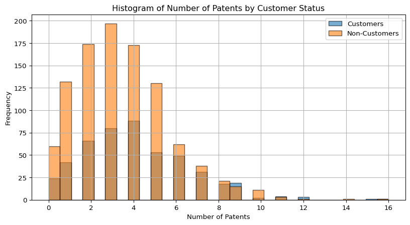

Customer Mean Number of Patents: 4.133056133056133
Non-Customer Mean Number of Patents: 3.4730127576054954

Customers tend to have a slightly higher frequency of companies with more patents compared to non-customers. The distribution for both groups is right-skewed, but the customer group has a longer tail toward higher patent counts. The average patents for customers is around 4.13 and the average patents for non-customers is around 3.47.

This suggests that customer companies, on average, have more patents than non-customers, possibly indicating greater innovation or R&D activity.

Blueprinty customers are not selected at random. It may be important to account for systematic differences in the age and regional location of customers vs non-customers.

We also then compare regions and ages by customer status.

import seaborn as sns
customers = df[df['iscustomer'] == 1]
non_customers = df[df['iscustomer'] == 0]

fig, axes = plt.subplots(1, 2, figsize=(14, 5))

sns.boxplot(data=df, x='iscustomer', y='age', ax=axes[0])
axes[0].set_title('Age by Customer Status')
axes[0].set_xticks([0, 1])
axes[0].set_xticklabels(['Non-Customers', 'Customers'])
axes[0].set_ylabel('Age')

region_counts = pd.crosstab(df['region'], df['iscustomer'])
sorted_regions = region_counts[1].sort_values(ascending=False).index
region_counts_sorted = region_counts.loc[sorted_regions]
region_counts_sorted.plot(kind='bar', stacked=False, ax=axes[1])
axes[1].set_title('Region Distribution by Customer Status')
axes[1].legend(title='Customer Status', labels=['Non-Customer', 'Customer'])
axes[1].set_ylabel('Counts')

plt.tight_layout()
plt.show()

mean_age_customers = customers['age'].mean()
mean_age_non_customers = non_customers['age'].mean()

customer_region_counts = region_counts[1].sort_values(ascending=False)

print(f'Customer Mean Age: {mean_age_customers}')
print(f'Non-Customer Mean Age:{mean_age_non_customers}')
print(f'Customer Region Counts:')
print('===============================')
customer_region_counts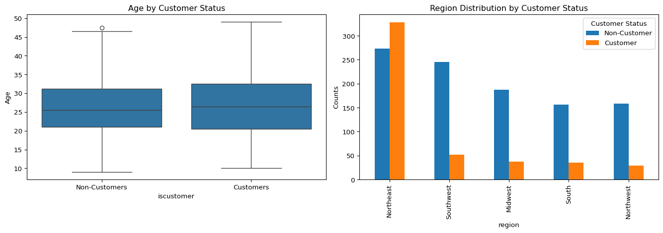

Customer Mean Age: 26.9002079002079
Non-Customer Mean Age:26.101570166830225
Customer Region Counts:
===============================

region
Northeast    328
Southwest     52
Midwest       37
South         35
Northwest     29
Name: 1, dtype: int64

Customers tend to be slightly older than non-customers, with a mean age of 26.9 compared to 26.1. The age distributions are similar overall, but customer firms show a slightly higher median and greater variability. Regionally, the Northeast stands out with the highest number of customer firms (328), while other regions such as the Southwest, Midwest, South, and Northwest have significantly fewer customers. This suggests that both firm age and geographic location may be associated with customer status, with the Northeast possibly representing a key market area.

Estimation of Simple Poisson Model

Since our outcome variable of interest can only be small integer values per a set unit of time, we can use a Poisson density to model the number of patents awarded to each engineering firm over the last 5 years. We start by estimating a simple Poisson model via Maximum Likelihood.

We assume that ( Y_1, Y_2, , Y_n () ). The probability mass function for each observation is:

\[ f(Y_i \mid \lambda) = \frac{e^{-\lambda} \lambda^{Y_i}}{Y_i!} \]

Assuming independence, the likelihood function for the sample is:

\[ L(\lambda; Y_1, \dots, Y_n) = \prod_{i=1}^n \frac{e^{-\lambda} \lambda^{Y_i}}{Y_i!} \]

This simplifies to:

\[ L(\lambda) = \frac{e^{-n\lambda} \lambda^{\sum Y_i}}{\prod Y_i!} \]

import numpy as np
from scipy.special import gammaln

def poisson_loglikelihood(lambda_, Y):
    if lambda_ <= 0:
        return -np.inf  
    return np.sum(Y * np.log(lambda_) - lambda_ - gammaln(Y + 1))

The function poisson_loglikelihood(lambda_, Y) calculates the log-likelihood of observing a dataset of counts (Y) under a Poisson distribution with rate parameter \(\lambda\). It assumes that the counts are independent and identically distributed. The function first checks whether \(\lambda\) is positive, since the Poisson rate must be greater than zero, and returns negative infinity if it is not. It then computes the log-likelihood by summing the terms (Y (\(\lambda\)) - \(\lambda\) - (Y!)) across all observations. The gammaln(Y + 1) function is used to compute ((Y!)) in a numerically stable way. This implementation is useful for estimating \(\lambda\) using maximum likelihood estimation.

We then use our function poisson_loglikelihood(lambda_, Y) to plot lambda on the horizontal axis and the log-likelihood on the vertical axis for a range of lambdas.

Y = df['patents']
lambda_values = np.linspace(0.1, 10, 200)
log_likelihoods = [poisson_loglikelihood(l, Y) for l in lambda_values]

plt.figure(figsize=(10, 6))
plt.plot(lambda_values, log_likelihoods, label='Log-Likelihood')
plt.xlabel('Lambda (λ)')
plt.ylabel('Log-Likelihood')
plt.title('Poisson Log-Likelihood vs. Lambda')
plt.grid(True)
plt.legend()
plt.show()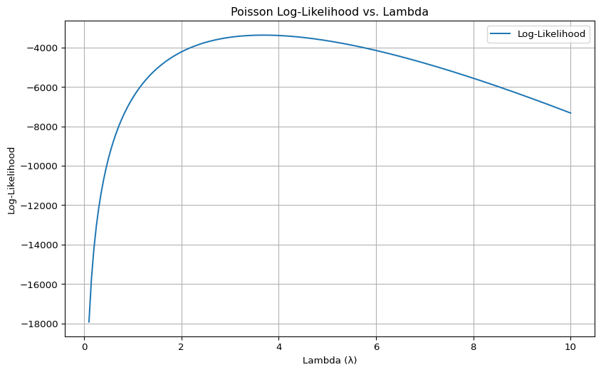

This plot shows the log likelihood function of a Poisson model for a range of \(\lambda\) values, using the observed number of patents as the input data. The horizontal axis represents different values of \(\lambda\), the rate parameter of the Poisson distribution, while the vertical axis shows the corresponding log likelihood values. The curve peaks at the value of \(\lambda\) that best fits the data, which is the maximum likelihood estimate (MLE). The shape of the curve illustrates how sensitive the likelihood is to changes in \(\lambda\), with values that are too low or too high producing a poorer fit. The MLE seems be around a \(\lambda\) value of 3.5.

Deriving the MLE for the Poisson Rate Parameter λ Given that the log-likelihood function is: \[ \ell(\lambda) = \sum_{i=1}^n \left( Y_i \log \lambda - \lambda - \log Y_i! \right) \] Take the derivative with respect to \(\lambda\): \[ \frac{d\ell}{d\lambda} = \sum_{i=1}^n \left( \frac{Y_i}{\lambda} - 1 \right) = \frac{1}{\lambda} \sum_{i=1}^n Y_i - n \] Set the derivative equal to 0: \[ \frac{1}{\lambda} \sum_{i=1}^n Y_i - n = 0 \] Solve for \(\lambda\): \[ \lambda = \frac{1}{n} \sum_{i=1}^n Y_i = \bar{Y} \] Therefore, the maximum likelihood estimator (MLE) for \(\lambda\) is the sample mean: \[ \lambda_{\text{MLE}} = \bar{Y} \]

from scipy.optimize import minimize

def neg_loglikelihood(lambda_, Y):
    return -poisson_loglikelihood(lambda_, Y)

initial_guess = [1.0]

result = minimize(neg_loglikelihood, x0=initial_guess, args=(Y,), bounds=[(0.01, None)])

lambda_mle = result.x[0]
print(f'Estimated MLE: {lambda_mle}')

Estimated MLE: 3.6846667021660804

The optimized MLE is approximately 3.68.

Estimation of Poisson Regression Model

Next, we extend our simple Poisson model to a Poisson Regression Model such that \(Y_i = \text{Poisson}(\lambda_i)\) where \(\lambda_i = \exp(X_i'\beta)\). The interpretation is that the success rate of patent awards is not constant across all firms (\(\lambda\)) but rather is a function of firm characteristics \(X_i\). Specifically, we will use the covariates age, age squared, region, and whether the firm is a customer of Blueprinty.

import numpy as np
from scipy.special import gammaln
import math

def poisson_regression_loglikelihood(beta, Y, X):
    # ensure shapes
    beta = np.asarray(beta).ravel()
    X = np.asarray(X)
    Y = np.asarray(Y)

    # linear predictor
    linpred = X.dot(beta)
    linpred = np.clip(linpred, -100, 100)   # avoid overflow

    # use math.exp for each element
    mu = np.array([math.exp(val) for val in linpred])

    if np.any(mu <= 0) or np.any(np.isnan(mu)):
        return -np.inf

    return np.sum(Y * np.log(mu) - mu - gammaln(Y + 1))

This function poisson_regression_loglikelihood(beta, Y, X) computes the log-likelihood for a Poisson regression model. Instead of assuming a constant rate \(\lambda\), it models the rate for each observation as \(\lambda_i = \exp(X_i' \beta)\), where \(X_i\) represents the covariates (such as age, region, and customer status) and \(\beta\) is the vector of coefficients. The function first calculates the linear predictor \(X \beta\), exponentiates it to obtain \(\lambda_i\), and then evaluates the log-likelihood by summing \(Y_i \log(lambda_i) - \lambda_i - \log(Y_i!)\) across all observations. This approach allows the expected count to vary across firms based on their characteristics.

We then use our function along with Python’s sp.optimize() to find the MLE vector and the Hessian of the Poisson model with covariates.

import numpy as np
import pandas as pd
from scipy.optimize import minimize
df['age_squared'] = df['age'] ** 2
region_dummies = pd.get_dummies(df['region'], drop_first=True)
X = pd.concat([
    pd.Series(1, index=df.index, name='intercept'),
    df[['age', 'age_squared', 'iscustomer']],
    region_dummies
], axis=1)
Y = df['patents'].values
X_matrix = X.values

def neg_loglikelihood(beta, Y, X):
    return -poisson_regression_loglikelihood(beta, Y, X)

initial_beta = np.zeros(X_matrix.shape[1])
result = minimize(neg_loglikelihood, x0=initial_beta, args=(Y, X_matrix), method='BFGS')

beta_mle = result.x
hess_inv = result.hess_inv

if not isinstance(hess_inv, np.ndarray):
    hess_inv = hess_inv.todense()
hess_inv = np.asarray(hess_inv)

std_errors = np.sqrt(np.diag(hess_inv))

results_df = pd.DataFrame({
    "Coefficient": beta_mle,
    "Std. Error": std_errors
}, index=X.columns)
results_df

	Coefficient	Std. Error
intercept	-0.509991	0.439064
age	0.148706	0.035334
age_squared	-0.002972	0.000681
iscustomer	0.207609	0.028506
Northeast	0.029155	0.034799
Northwest	-0.017578	0.045014
South	0.056565	0.043264
Southwest	0.050567	0.035334

We then check our results with Python’s sm.GLM() function.

import statsmodels.api as sm

X_numeric = X.astype(float)
Y_numeric = Y.astype(float)

poisson_model = sm.GLM(Y_numeric, X_numeric, family=sm.families.Poisson())
poisson_results = poisson_model.fit()
print(poisson_results.summary())

import pandas as pd
result_table = pd.DataFrame({
    'coef': poisson_results.params,
    'std_err': poisson_results.bse
})
print(result_table)

                 Generalized Linear Model Regression Results                  
==============================================================================
Dep. Variable:                      y   No. Observations:                 1500
Model:                            GLM   Df Residuals:                     1492
Model Family:                 Poisson   Df Model:                            7
Link Function:                    Log   Scale:                          1.0000
Method:                          IRLS   Log-Likelihood:                -3258.1
Date:                Wed, 07 May 2025   Deviance:                       2143.3
Time:                        22:43:16   Pearson chi2:                 2.07e+03
No. Iterations:                     5   Pseudo R-squ. (CS):             0.1360
Covariance Type:            nonrobust                                         
===============================================================================
                  coef    std err          z      P>|z|      [0.025      0.975]
-------------------------------------------------------------------------------
intercept      -0.5089      0.183     -2.778      0.005      -0.868      -0.150
age             0.1486      0.014     10.716      0.000       0.121       0.176
age_squared    -0.0030      0.000    -11.513      0.000      -0.003      -0.002
iscustomer      0.2076      0.031      6.719      0.000       0.147       0.268
Northeast       0.0292      0.044      0.669      0.504      -0.056       0.115
Northwest      -0.0176      0.054     -0.327      0.744      -0.123       0.088
South           0.0566      0.053      1.074      0.283      -0.047       0.160
Southwest       0.0506      0.047      1.072      0.284      -0.042       0.143
===============================================================================
                 coef   std_err
intercept   -0.508920  0.183179
age          0.148619  0.013869
age_squared -0.002970  0.000258
iscustomer   0.207591  0.030895
Northeast    0.029170  0.043625
Northwest   -0.017575  0.053781
South        0.056561  0.052662
Southwest    0.050576  0.047198

Age has a strong nonlinear relationship with patent counts: each additional year of firm age increases the expected log count (coefficient 0.149, p < .001), but the negative age squared term (coefficient –0.003, p < .001) means that this benefit tapers off around 25 years of age before declining. Firms that are Blueprinty customers produce about 23 percent more patents than non-customers (exp(0.208)≈1.23, p < .001), all else equal. Once age and customer status are accounted for, none of the regions—Northeast, Northwest, South, or Southwest—differs significantly from the Midwest baseline. The model’s Cragg & Uhler pseudo R² of 0.136 indicates these predictors explain roughly 13.6 percent of the variation in patent counts.

X_base = pd.concat([
    pd.Series(1, index=df.index, name='intercept'),
    df[['age', 'age_squared']],
    region_dummies
], axis=1)

X_0 = X_base.copy()
X_0['iscustomer'] = 0
X_0 = X_0[['intercept', 'age', 'age_squared', 'iscustomer'] + list(region_dummies.columns)]

X_1 = X_base.copy()
X_1['iscustomer'] = 1
X_1 = X_1[['intercept', 'age', 'age_squared', 'iscustomer'] + list(region_dummies.columns)]

X_full = X_base.copy()
X_full['iscustomer'] = df['iscustomer']
X_full = X_full[['intercept', 'age', 'age_squared', 'iscustomer'] + list(region_dummies.columns)]

Y = df['patents'].astype(float)

model = sm.GLM(Y, X_full.astype(float), family=sm.families.Poisson())
result = model.fit()

y_pred_0 = result.predict(X_0.astype(float))
y_pred_1 = result.predict(X_1.astype(float))

average_effect = np.mean(y_pred_1 - y_pred_0)
average_effect

np.float64(0.7927680710452699)

The analysis shows that, on average, firms predicted to be Blueprinty customers are expected to produce approximately 0.79 more patents than if they were not customers, holding all other firm characteristics constant.

AirBnB Case Study

Introduction

AirBnB is a popular platform for booking short-term rentals. In March 2017, students Annika Awad, Evan Lebo, and Anna Linden scraped of 40,000 Airbnb listings from New York City. The data include the following variables:

Variable Definitions

- `id` = unique ID number for each unit
- `last_scraped` = date when information scraped
- `host_since` = date when host first listed the unit on Airbnb
- `days` = `last_scraped` - `host_since` = number of days the unit has been listed
- `room_type` = Entire home/apt., Private room, or Shared room
- `bathrooms` = number of bathrooms
- `bedrooms` = number of bedrooms
- `price` = price per night (dollars)
- `number_of_reviews` = number of reviews for the unit on Airbnb
- `review_scores_cleanliness` = a cleanliness score from reviews (1-10)
- `review_scores_location` = a "quality of location" score from reviews (1-10)
- `review_scores_value` = a "quality of value" score from reviews (1-10)
- `instant_bookable` = "t" if instantly bookable, "f" if not

EDA:

df = pd.read_csv("airbnb.csv")
df.describe(include='all')

	Unnamed: 0	id	days	last_scraped	host_since	room_type	bathrooms	bedrooms	price	number_of_reviews	review_scores_cleanliness	review_scores_location	review_scores_value	instant_bookable
count	40628.000000	4.062800e+04	40628.000000	40628	40593	40628	40468.000000	40552.000000	40628.000000	40628.000000	30433.000000	30374.000000	30372.000000	40628
unique	NaN	NaN	NaN	2	2790	3	NaN	NaN	NaN	NaN	NaN	NaN	NaN	2
top	NaN	NaN	NaN	4/2/2017	12/21/2015	Entire home/apt	NaN	NaN	NaN	NaN	NaN	NaN	NaN	f
freq	NaN	NaN	NaN	25737	65	19873	NaN	NaN	NaN	NaN	NaN	NaN	NaN	32759
mean	20314.500000	9.698889e+06	1102.368219	NaN	NaN	NaN	1.124592	1.147046	144.760732	15.904426	9.198370	9.413544	9.331522	NaN
std	11728.437705	5.460166e+06	1383.269358	NaN	NaN	NaN	0.385884	0.691746	210.657597	29.246009	1.119935	0.844949	0.902966	NaN
min	1.000000	2.515000e+03	1.000000	NaN	NaN	NaN	0.000000	0.000000	10.000000	0.000000	2.000000	2.000000	2.000000	NaN
25%	10157.750000	4.889868e+06	542.000000	NaN	NaN	NaN	1.000000	1.000000	70.000000	1.000000	9.000000	9.000000	9.000000	NaN
50%	20314.500000	9.862878e+06	996.000000	NaN	NaN	NaN	1.000000	1.000000	100.000000	4.000000	10.000000	10.000000	10.000000	NaN
75%	30471.250000	1.466789e+07	1535.000000	NaN	NaN	NaN	1.000000	1.000000	170.000000	17.000000	10.000000	10.000000	10.000000	NaN
max	40628.000000	1.800967e+07	42828.000000	NaN	NaN	NaN	8.000000	10.000000	10000.000000	421.000000	10.000000	10.000000	10.000000	NaN

missing_values = df.isna().sum()

missing_values = missing_values[missing_values > 0]

plt.figure(figsize=(10, 6))
missing_values.plot(kind='bar')
plt.title('Missing Values per Column')
plt.xlabel('Columns')
plt.ylabel('Number of Missing Values')
plt.xticks(rotation=45)
plt.grid(axis='y')
plt.tight_layout()
plt.show()

print("Missing Values:")
print(missing_values)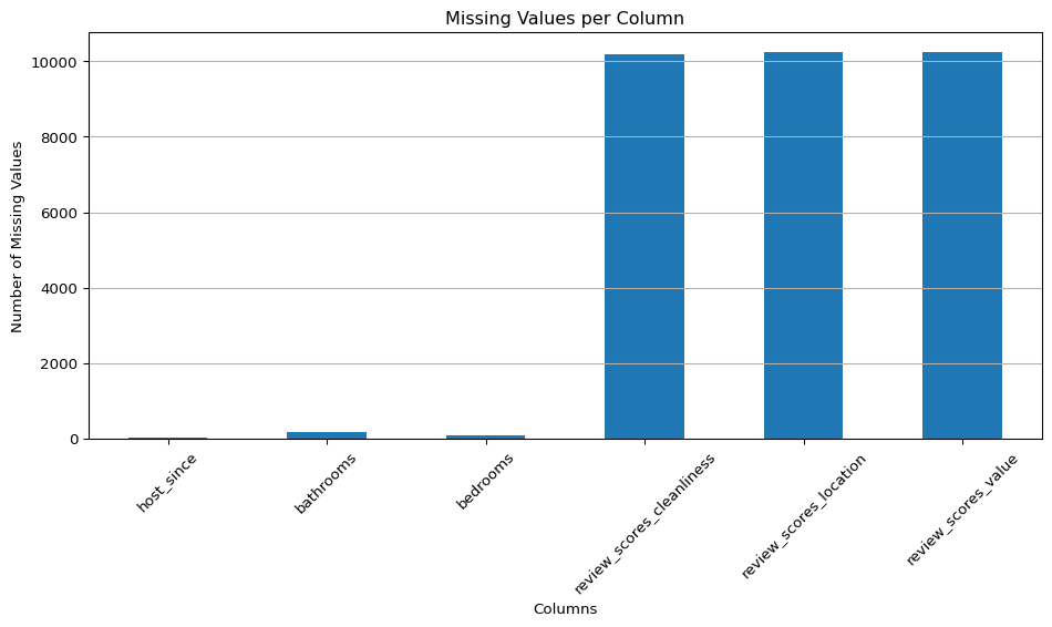

Missing Values:
host_since                      35
bathrooms                      160
bedrooms                        76
review_scores_cleanliness    10195
review_scores_location       10254
review_scores_value          10256
dtype: int64

host_since: 35 missing
bathrooms: 160 missing
bedrooms: 76 missing
cleanliness: 10,195 missing
location: 10,254 missing
value: 10,256 missing

We then built a poisson regression model for the number of bookings as proxied by the number of reviews.

columns_required = [
    'days', 'room_type', 'bathrooms', 'bedrooms', 'price',
    'review_scores_cleanliness', 'review_scores_location',
    'review_scores_value', 'instant_bookable', 'number_of_reviews'
]
df_clean = df.dropna(subset=columns_required)

df_clean = pd.get_dummies(df_clean, columns=['room_type', 'instant_bookable'], drop_first=True)

X = df_clean[[
    'days', 'bathrooms', 'bedrooms', 'price',
    'review_scores_cleanliness', 'review_scores_location', 'review_scores_value',
    'room_type_Private room', 'room_type_Shared room', 'instant_bookable_t'
]]
X = sm.add_constant(X)  
Y = df_clean['number_of_reviews']

X = X.astype(float)
Y = Y.astype(float)

model = sm.GLM(Y, X, family=sm.families.Poisson())
result = model.fit()

results_df = pd.DataFrame({
    'Coefficient': result.params,
    'Std. Error': result.bse
})
print(results_df)

                           Coefficient    Std. Error
const                         3.498049  1.609066e-02
days                          0.000051  3.909218e-07
bathrooms                    -0.117704  3.749225e-03
bedrooms                      0.074087  1.991742e-03
price                        -0.000018  8.326458e-06
review_scores_cleanliness     0.113139  1.496336e-03
review_scores_location       -0.076899  1.608903e-03
review_scores_value          -0.091076  1.803855e-03
room_type_Private room       -0.010536  2.738448e-03
room_type_Shared room        -0.246337  8.619793e-03
instant_bookable_t            0.345850  2.890138e-03

We dropped rows with missing values for modeling, created dummy variables for room_type and instant_bookable, and fit a Poisson regression model with number_of_reviews as the outcome.

Observations: - Intercept (3.50): - This is the expected log number of reviews for a listing with all predictors at zero. While not directly interpretable on its own, it anchors the model.

days (0.0000507):
- For each additional day a listing is on the platform, the expected number of reviews increases slightly. Since the coefficient is small, the cumulative effect builds over time.
bathrooms (–0.118):
- More bathrooms are associated with fewer reviews, holding everything else constant. This may indicate that listings with more bathrooms (likely larger or higher-end) receive fewer but possibly higher-value bookings.
bedrooms (0.074):
- Each additional bedroom is associated with more reviews, suggesting larger units are booked more frequently.
price (–0.0000179):
- Higher nightly prices are associated with fewer reviews, as expected. Though small per dollar, the effect accumulates for expensive listings.
Cleanliness (0.113):
- Higher cleanliness scores significantly increase the number of reviews, reflecting the value guests place on a clean space.
Value (–0.077) and Location (–0.091):
- Interestingly, higher value and location scores are slightly negatively associated with review counts, possibly reflecting more niche or stable listings that receive fewer but more favorable reviews.
Private Room (–0.0105):
- Compared to entire homes, private rooms receive slightly fewer reviews.
Shared Room (–0.247):
- Shared rooms receive significantly fewer reviews, suggesting they are much less popular among guests.