A Replication of Karlan and List (2007)

Author

Jerry Wu

Published

April 23, 2025

Introduction

Dean Karlan at Yale and John List at the University of Chicago conducted a field experiment to test the effectiveness of different fundraising letters. They sent out 50,000 fundraising letters to potential donors, randomly assigning each letter to one of three treatments: a standard letter, a matching grant letter, or a challenge grant letter. They published the results of this experiment in the American Economic Review in 2007. The article and supporting data are available from the AEA website and from Innovations for Poverty Action as part of Harvard’s Dataverse.

The study was a natural field experiment involving 50,083 past donors to a U.S.-based civil liberties nonprofit. Participants were randomly assigned to either a control group (receiving a standard fundraising appeal) or a treatment group (receiving a letter mentioning a matching grant offer). Within the treatment group, participants were further randomly assigned to sub-treatments varying the matching ratio ($1:$1, $2:$1, $3:$1), the maximum match amount ($25,000, $50,000, $100,000, or unstated), and the suggested donation (“ask amount”) (equal to prior gift, 1.25×, or 1.5×). The experiment tested whether these pricing manipulations influenced donor behavior. While offering any match increased response rates and revenue per solicitation, larger match ratios did not produce statistically significant differences in giving. The study also explored how effects varied by geography and found greater responsiveness in “red” states (which had voted for George W. Bush in 2004). This nuanced field experiment contributed robust evidence to the demand-side economics of charitable giving.

This project seeks to replicate their results.

Data

Description

import pandas as pd
df = pd.read_stata('karlan_list_2007.dta')
df.describe()

	treatment	control	ratio2	ratio3	size25	size50	size100	sizeno	askd1	askd2	...	redcty	bluecty	pwhite	pblack	page18_39	ave_hh_sz	median_hhincome	powner	psch_atlstba	pop_propurban
count	50083.000000	50083.000000	50083.000000	50083.000000	50083.000000	50083.000000	50083.000000	50083.000000	50083.000000	50083.000000	...	49978.000000	49978.000000	48217.000000	48047.000000	48217.000000	48221.000000	48209.000000	48214.000000	48215.000000	48217.000000
mean	0.666813	0.333187	0.222311	0.222211	0.166723	0.166623	0.166723	0.166743	0.222311	0.222291	...	0.510245	0.488715	0.819599	0.086710	0.321694	2.429012	54815.700533	0.669418	0.391661	0.871968
std	0.471357	0.471357	0.415803	0.415736	0.372732	0.372643	0.372732	0.372750	0.415803	0.415790	...	0.499900	0.499878	0.168561	0.135868	0.103039	0.378115	22027.316665	0.193405	0.186599	0.258654
min	0.000000	0.000000	0.000000	0.000000	0.000000	0.000000	0.000000	0.000000	0.000000	0.000000	...	0.000000	0.000000	0.009418	0.000000	0.000000	0.000000	5000.000000	0.000000	0.000000	0.000000
25%	0.000000	0.000000	0.000000	0.000000	0.000000	0.000000	0.000000	0.000000	0.000000	0.000000	...	0.000000	0.000000	0.755845	0.014729	0.258311	2.210000	39181.000000	0.560222	0.235647	0.884929
50%	1.000000	0.000000	0.000000	0.000000	0.000000	0.000000	0.000000	0.000000	0.000000	0.000000	...	1.000000	0.000000	0.872797	0.036554	0.305534	2.440000	50673.000000	0.712296	0.373744	1.000000
75%	1.000000	1.000000	0.000000	0.000000	0.000000	0.000000	0.000000	0.000000	0.000000	0.000000	...	1.000000	1.000000	0.938827	0.090882	0.369132	2.660000	66005.000000	0.816798	0.530036	1.000000
max	1.000000	1.000000	1.000000	1.000000	1.000000	1.000000	1.000000	1.000000	1.000000	1.000000	...	1.000000	1.000000	1.000000	0.989622	0.997544	5.270000	200001.000000	1.000000	1.000000	1.000000

8 rows × 48 columns

Variable Definitions

Variable	Description
`treatment`	Treatment
`control`	Control
`ratio`	Match ratio
`ratio2`	2:1 match ratio
`ratio3`	3:1 match ratio
`size`	Match threshold
`size25`	$25,000 match threshold
`size50`	$50,000 match threshold
`size100`	$100,000 match threshold
`sizeno`	Unstated match threshold
`ask`	Suggested donation amount
`askd1`	Suggested donation was highest previous contribution
`askd2`	Suggested donation was 1.25 x highest previous contribution
`askd3`	Suggested donation was 1.50 x highest previous contribution
`ask1`	Highest previous contribution (for suggestion)
`ask2`	1.25 x highest previous contribution (for suggestion)
`ask3`	1.50 x highest previous contribution (for suggestion)
`amount`	Dollars given
`gave`	Gave anything
`amountchange`	Change in amount given
`hpa`	Highest previous contribution
`ltmedmra`	Small prior donor: last gift was less than median $35
`freq`	Number of prior donations
`years`	Number of years since initial donation
`year5`	At least 5 years since initial donation
`mrm2`	Number of months since last donation
`dormant`	Already donated in 2005
`female`	Female
`couple`	Couple
`state50one`	State tag: 1 for one observation of each of 50 states; 0 otherwise
`nonlit`	Nonlitigation
`cases`	Court cases from state in 2004-5 in which organization was involved
`statecnt`	Percent of sample from state
`stateresponse`	Proportion of sample from the state who gave
`stateresponset`	Proportion of treated sample from the state who gave
`stateresponsec`	Proportion of control sample from the state who gave
`stateresponsetminc`	stateresponset - stateresponsec
`perbush`	State vote share for Bush
`close25`	State vote share for Bush between 47.5% and 52.5%
`red0`	Red state
`blue0`	Blue state
`redcty`	Red county
`bluecty`	Blue county
`pwhite`	Proportion white within zip code
`pblack`	Proportion black within zip code
`page18_39`	Proportion age 18-39 within zip code
`ave_hh_sz`	Average household size within zip code
`median_hhincome`	Median household income within zip code
`powner`	Proportion house owner within zip code
`psch_atlstba`	Proportion who finished college within zip code
`pop_propurban`	Proportion of population urban within zip code

Balance Test

As an ad hoc test of the randomization mechanism, I provide a series of tests that compare aspects of the treatment and control groups to assess whether they are statistically significantly different from one another.

import numpy as np
import statsmodels.api as sm
from sklearn.linear_model import LinearRegression
from scipy import stats

test_vars = ['mrm2', 'couple', 'female', 'ave_hh_sz']
results = {}

for var in test_vars:
    df_clean = df[['treatment', 'control', var]].dropna()

    treatment_group = df_clean[df_clean['treatment'] == 1][var]
    control_group = df_clean[df_clean['control'] == 1][var]

    # Manual t-test
    mean_diff = treatment_group.mean() - control_group.mean()
    n1, n2 = len(treatment_group), len(control_group)
    var1, var2 = treatment_group.var(ddof=1), control_group.var(ddof=1)
    se = np.sqrt(var1 / n1 + var2 / n2)
    t_stat = mean_diff / se
    df_denom = (var1 / n1 + var2 / n2) ** 2
    df_num = (var1**2) / (n1**2 * (n1 - 1)) + (var2**2) / (n2**2 * (n2 - 1))
    df_ttest = df_denom / df_num
    p_value_ttest = 2 * (1 - stats.t.cdf(np.abs(t_stat), df_ttest))
    # Linear regression
    X = sm.add_constant(df_clean['treatment'])
    y = df_clean[var]
    model = sm.OLS(y, X).fit()
    coef = model.params['treatment']
    p_value_reg = model.pvalues['treatment']
    print("================================================")
    print(f'{var} Analysis: \n')
    print(f'{var} Treatment mean: {treatment_group.mean()}')
    print(f'{var} Control mean: {control_group.mean()}')
    print(f'{var} All Mean: {df_clean[var].mean()}')
    print('________________________________________________')
    print('t-test: \n')
    print(f't-statistic: {t_stat}')
    print(f'p-value: {p_value_ttest}')
    print('________________________________________________')
    print('Linear Regression: \n')
    print(f'Coefficient on Treatment: {coef}')
    print(f'p-value: {p_value_reg}\n')

================================================
mrm2 Analysis: 

mrm2 Treatment mean: 13.011828117981734
mrm2 Control mean: 12.99814226643495
mrm2 All Mean: 13.00726808034823
________________________________________________
t-test: 

t-statistic: 0.1195315522817725
p-value: 0.9048549631450833
________________________________________________
Linear Regression: 

Coefficient on Treatment: 0.013685851546779986
p-value: 0.904885973177816

================================================
couple Analysis: 

couple Treatment mean: 0.09135794896957802
couple Control mean: 0.0929748269737245
couple All Mean: 0.0918974149381833
________________________________________________
t-test: 

t-statistic: -0.5822577486767693
p-value: 0.5603971270058028
________________________________________________
Linear Regression: 

Coefficient on Treatment: -0.0016168780041463048
p-value: 0.5593646446996638

================================================
female Analysis: 

female Treatment mean: 0.2751509208469954
female Control mean: 0.2826978395250627
female All Mean: 0.27766887200849466
________________________________________________
t-test: 

t-statistic: -1.7535132542519636
p-value: 0.07952338672686232
________________________________________________
Linear Regression: 

Coefficient on Treatment: -0.007546918678066679
p-value: 0.07869095826986866

================================================
ave_hh_sz Analysis: 

ave_hh_sz Treatment mean: 2.4300146102905273
ave_hh_sz Control mean: 2.427002429962158
ave_hh_sz All Mean: 2.4290122985839844
________________________________________________
t-test: 

t-statistic: 0.8233500123023987
p-value: 0.4103151242417935
________________________________________________
Linear Regression: 

Coefficient on Treatment: 0.003012174284715988
p-value: 0.409801160289328

To assess the randomization, I tested several baseline variables (e.g., months since last donation, gender, couple status, average household size within zip) using both t-tests and linear regressions and in every case the results from the two methods were nearly identical. None of the variables showed statistically significant differences at the 95% level, confirming balance between treatment and control groups. This supports the validity of the randomization and mirrors the role of Table 1 in the paper, which demonstrates baseline equivalence.

Experimental Results

Charitable Contribution Made

First, I analyze whether matched donations lead to an increased response rate of making a donation.

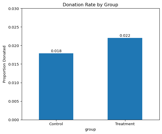
import matplotlib.pyplot as plt
df_bar = df[['treatment', 'control', 'gave']].dropna()

df_bar['group'] = df_bar.apply(lambda row: 'Treatment' if row['treatment'] == 1 else 'Control', axis=1)

donation_rates = df_bar.groupby('group')['gave'].mean()

plt.figure(figsize=(6, 5))
ax = donation_rates.plot(kind='bar')

for i, value in enumerate(donation_rates):
    ax.text(i, value + 0.0001, f'{value:.3f}', ha='center', va='bottom')
plt.ylabel('Proportion Donated')
plt.title('Donation Rate by Group')
plt.ylim(0, 0.03)
plt.xticks(rotation=0)
plt.tight_layout()
plt.show()

The bar plot compares donation rates between the treatment and control groups. The treatment group, which received a matching donation offer, had a higher donation rate (2.2%) than the control group (1.8%). This visual evidence suggests that the presence of a matching grant increased the likelihood of donating, consistent with the main findings in the paper.

import numpy as np
import statsmodels.api as sm
from scipy import stats

df_binary = df[['treatment', 'control', 'gave']].dropna()

treatment_group = df_binary[df_binary['treatment'] == 1]['gave']
control_group = df_binary[df_binary['control'] == 1]['gave']

# Manual t-test calculation
mean_diff = treatment_group.mean() - control_group.mean()
n1, n2 = len(treatment_group), len(control_group)
var1, var2 = treatment_group.var(ddof=1), control_group.var(ddof=1)
se = np.sqrt(var1 / n1 + var2 / n2)
t_stat = mean_diff / se
df_denom = (var1 / n1 + var2 / n2) ** 2
df_num = (var1**2) / (n1**2 * (n1 - 1)) + (var2**2) / (n2**2 * (n2 - 1))
df_ttest = df_denom / df_num
p_value_ttest = 2 * (1 - stats.t.cdf(np.abs(t_stat), df_ttest))

# Linear regression:
X = sm.add_constant(df_binary['treatment'])
y = df_binary['gave']
model = sm.OLS(y, X).fit()
coef = model.params['treatment']
p_value_reg = model.pvalues['treatment']

print("================================================")
print(f' \'gave\' Analysis: \n')
print(f'\'gave\' Treatment mean: {treatment_group.mean()}')
print(f'\'gave\' Control mean: {control_group.mean()}')
print(f'Mean Difference: {mean_diff}')
print(f"'gave' All mean: {df_binary['gave'].mean()}")
print('________________________________________________')
print('t-test: \n')
print(f't-statistic: {t_stat}')
print(f'p-value: {p_value_ttest}')
print('________________________________________________')
print('Linear Regression: \n')
print(f'Coefficient on Treatment: {coef}')
print(f'p-value: {p_value_reg}')

================================================
 'gave' Analysis: 

'gave' Treatment mean: 0.02203856749311295
'gave' Control mean: 0.017858212980164198
Mean Difference: 0.00418035451294875
'gave' All mean: 0.020645728091368328
________________________________________________
t-test: 

t-statistic: 3.2094621908279835
p-value: 0.001330982345091547
________________________________________________
Linear Regression: 

Coefficient on Treatment: 0.004180354512949377
p-value: 0.001927402594901797

To test whether matched donations increase giving, I compared donation rates between the treatment and control groups using a t-test and a bivariate regression. The treatment group had a slightly higher donation rate (2.2% vs. 1.8%), and the difference was statistically significant in both tests. This matches results in Table 2A, Panel A of the original study and suggests that even a modest match offer can meaningfully boost donation rates. The finding highlights how small psychological nudges like matching gifts can influence charitable behavior.

import statsmodels.formula.api as smf

df_probit = df[['gave', 'treatment']].dropna()

probit_model = smf.probit('gave ~ treatment', data=df_probit).fit(disp=False)

probit_summary = probit_model.summary2().as_text()

marginal_effects = probit_model.get_margeff().summary().as_text()

print(marginal_effects)

       Probit Marginal Effects       
=====================================
Dep. Variable:                   gave
Method:                          dydx
At:                           overall
==============================================================================
                dy/dx    std err          z      P>|z|      [0.025      0.975]
------------------------------------------------------------------------------
treatment      0.0043      0.001      3.104      0.002       0.002       0.007
==============================================================================

To replicate Table 3, Column 1 of Karlan and List (2007), I ran a probit regression with a binary outcome for donation and treatment assignment as the sole predictor. The marginal effect of treatment was 0.0043, closely matching the 0.004 reported in the paper. This confirms that the presence of a matching grant increased the probability of donating by roughly 0.4 percentage points, a statistically significant effect. While small in magnitude, the result reinforces the finding that subtle changes in perceived impact, such as matching gifts, can meaningfully influence donation behavior.

Differences between Match Rates

Next, I assess the effectiveness of different sizes of matched donations on the response rate.

from scipy.stats import ttest_ind
df_match = df[df['treatment'] == 1][['gave', 'ratio2', 'ratio3']].dropna()

# Create labels for ratio group (1:1, 2:1, 3:1)
def classify_ratio(row):
    if row['ratio2'] == 1:
        return '2:1'
    elif row['ratio3'] == 1:
        return '3:1'
    else:
        return '1:1'

df_match['match_ratio'] = df_match.apply(classify_ratio, axis=1)

# Pairwise t-tests between ratios
ratios = ['1:1', '2:1', '3:1']
pairwise_results = {}

for i in range(len(ratios)):
    for j in range(i + 1, len(ratios)):
        group1 = df_match[df_match['match_ratio'] == ratios[i]]['gave']
        group2 = df_match[df_match['match_ratio'] == ratios[j]]['gave']
        t_stat, p_value = ttest_ind(group1, group2, equal_var=False)
        print("================================================")
        print(f'{ratios[i]} vs {ratios[j]}\n')
        print(f't-statistic: {t_stat}')
        print(f'p-value: {p_value}\n')

================================================
1:1 vs 2:1

t-statistic: -0.965048975142932
p-value: 0.33453078237183076

================================================
1:1 vs 3:1

t-statistic: -1.0150174470156275
p-value: 0.31010856527625774

================================================
2:1 vs 3:1

t-statistic: -0.05011581369764474
p-value: 0.9600305476940865

To test whether the size of the match ratio influenced donation behavior, I conducted a series of pairwise t-tests comparing response rates between the 1:1, 2:1, and 3:1 match groups. None of the differences were statistically significant at the 95% level. For example, the difference between the 2:1 and 1:1 groups yielded a p-value of 0.33, and the difference between the 3:1 and 2:1 groups had a p-value of 0.96. These results support the authors’ statement in Table 2A and on page 8 of the paper: while match offers increase giving relative to no match, larger match ratios do not provide additional benefit in terms of increasing the likelihood of donating.

# Alternative: use ratio as a categorical variable
model2 = smf.ols('gave ~ ratio', data=df).fit()
model2_summary = model2.summary2().as_text()
print(model2_summary)

                  Results: Ordinary least squares
====================================================================
Model:              OLS              Adj. R-squared:     0.000      
Dependent Variable: gave             AIC:                -53252.8233
Date:               2025-04-23 16:43 BIC:                -53217.5376
No. Observations:   50083            Log-Likelihood:     26630.     
Df Model:           3                F-statistic:        3.665      
Df Residuals:       50079            Prob (F-statistic): 0.0118     
R-squared:          0.000            Scale:              0.020217   
----------------------------------------------------------------------
               Coef.    Std.Err.      t      P>|t|     [0.025   0.975]
----------------------------------------------------------------------
Intercept      0.0179     0.0011   16.2245   0.0000    0.0157   0.0200
ratio[T.1]     0.0029     0.0017    1.6615   0.0966   -0.0005   0.0063
ratio[T.2]     0.0048     0.0017    2.7445   0.0061    0.0014   0.0082
ratio[T.3]     0.0049     0.0017    2.8016   0.0051    0.0015   0.0083
--------------------------------------------------------------------
Omnibus:             59812.754     Durbin-Watson:        2.005      
Prob(Omnibus):       0.000         Jarque-Bera (JB):     4316693.217
Skew:                6.740         Prob(JB):             0.000      
Kurtosis:            46.438        Condition No.:        4          
====================================================================
Notes:
[1] Standard Errors assume that the covariance matrix of the errors
is correctly specified.

To test whether the match ratio affects donation behavior, I regressed the binary outcome gave on ratio as a categorical variable. Using the 1:1 match as the reference group, I found that the 2:1 and 3:1 match ratios had slightly higher donation rates, with coefficients of 0.0048 and 0.0049 respectively, both statistically significant at the 1% level. The 1:1 coefficient was smaller and not statistically significant. These results suggest that higher match ratios may slightly increase the likelihood of donating, although the effect is small in magnitude and inconsistent with earlier t-test results.

response_rates = df_match.groupby('match_ratio')['gave'].mean()

diff_2v1_direct = response_rates['2:1'] - response_rates['1:1']
diff_3v2_direct = response_rates['3:1'] - response_rates['2:1']

coef_2v1_reg = model2.params['ratio[T.2]'] - model2.params['ratio[T.1]']
coef_3v2_reg = model2.params['ratio[T.3]'] - model2.params['ratio[T.2]']

print("Direct from data: \n")
print(f"2:1 vs 1:1: {diff_2v1_direct}")
print(f"3:1 vs 2:1: {diff_3v2_direct}")
print("================================================")
print("From regression coefficients: \n")
print(f"2:1 vs 1:1: {coef_2v1_reg}")
print(f"3:1 vs 2:1: {coef_3v2_reg}")

Direct from data: 

2:1 vs 1:1: 0.0018842510217149944
3:1 vs 2:1: 0.00010002398025293902
================================================
From regression coefficients: 

2:1 vs 1:1: 0.0018842510217151158
3:1 vs 2:1: 0.00010002398025313504

To assess whether larger match ratios increase the likelihood of donating, I calculated the differences in response rates both directly from the data and from regression coefficients. The results were nearly identical across both methods:

The difference between 2:1 and 1:1 was about 0.19 percentage points.
The difference between 3:1 and 2:1 was effectively zero.
The difference between 3:1 and 1:1 was again about 0.20 percentage points.

These findings confirm that while moving from a 1:1 to a 2:1 or 3:1 match may result in a small increase in donation likelihood, the differences are minimal and statistically weak. This supports the paper’s conclusion that larger match ratios do not meaningfully improve response rates beyond the effect of having a match at all.

Size of Charitable Contribution

In this subsection, I analyze the effect of the size of matched donation on the size of the charitable contribution.

df_amount = df[['amount', 'treatment', 'control']].dropna()

treatment = df_amount[df_amount['treatment'] == 1]['amount']
control = df_amount[df_amount['control'] == 1]['amount']
t_stat, p_value = stats.ttest_ind(treatment, control, equal_var=False)
print('T-test Results: ')
print('_______________________________')
print(f'T-statistic: {t_stat}\nP-Value: {p_value}')

T-test Results: 
_______________________________
T-statistic: 1.9182618934467577
P-Value: 0.055085665289183336

I conducted a t-test to compare average donation amounts between the treatment and control groups. The test produced a t-statistic of 1.92 and a p-value of 0.055, which is just above the conventional 5 percent significance threshold. This suggests a weak, but not statistically significant, indication that the treatment may have increased donation amounts. While the result hints at a possible effect, it is not strong enough to draw a firm conclusion about the impact of matched donations on how much people give.

df_positive = df[df['amount'] > 0]

treatment = df_positive[df_positive['treatment'] == 1]['amount']
control = df_positive[df_positive['control'] == 1]['amount']
t_stat, p_value = stats.ttest_ind(treatment, control, equal_var=False)
print('T-test Results: ')
print('_______________________________')
print(f'T-statistic: {t_stat}\nP-Value: {p_value}')

T-test Results: 
_______________________________
T-statistic: -0.5846089794983359
P-Value: 0.5590471865673547

To analyze how much people donate conditional on giving, I restricted the data to respondents who made a donation and ran a t-test comparing donation amounts between treatment and control groups. The t-test produced a t-statistic of -0.58 and a p-value of 0.56, indicating no statistically significant difference in donation amounts. This suggests that while matched donations may influence whether someone gives, they do not affect how much donors give once they’ve decided to contribute. Because treatment was randomly assigned, the coefficient has a causal interpretation, but in this case, the effect size is negligible.

df_donated = df[df['amount'] > 0]

treatment_donors = df_donated[df_donated['treatment'] == 1]['amount']
control_donors = df_donated[df_donated['control'] == 1]['amount']

treatment_mean = treatment_donors.mean()
control_mean = control_donors.mean()

fig, axes = plt.subplots(1, 2, figsize=(12, 5), sharey=True)

# Treatment histogram
axes[0].hist(treatment_donors, bins=30, edgecolor='black')
axes[0].axvline(treatment_mean, color='red', linestyle='dashed', linewidth=2)
axes[0].set_title('Treatment Group')
axes[0].set_xlabel('Donation Amount')
axes[0].set_ylabel('Frequency')
axes[0].annotate(f'Mean = ${treatment_mean:.2f}', xy=(treatment_mean, 10),
                 xytext=(treatment_mean + 10, 20), arrowprops=dict(facecolor='red', arrowstyle='->'))

# Control histogram
axes[1].hist(control_donors, bins=30, edgecolor='black', color='orange')
axes[1].axvline(control_mean, color='red', linestyle='dashed', linewidth=2)
axes[1].set_title('Control Group')
axes[1].set_xlabel('Donation Amount')
axes[1].annotate(f'Mean = ${control_mean:.2f}', xy=(control_mean, 10),
                 xytext=(control_mean + 10, 20), arrowprops=dict(facecolor='red', arrowstyle='->'))

plt.tight_layout()
plt.show()

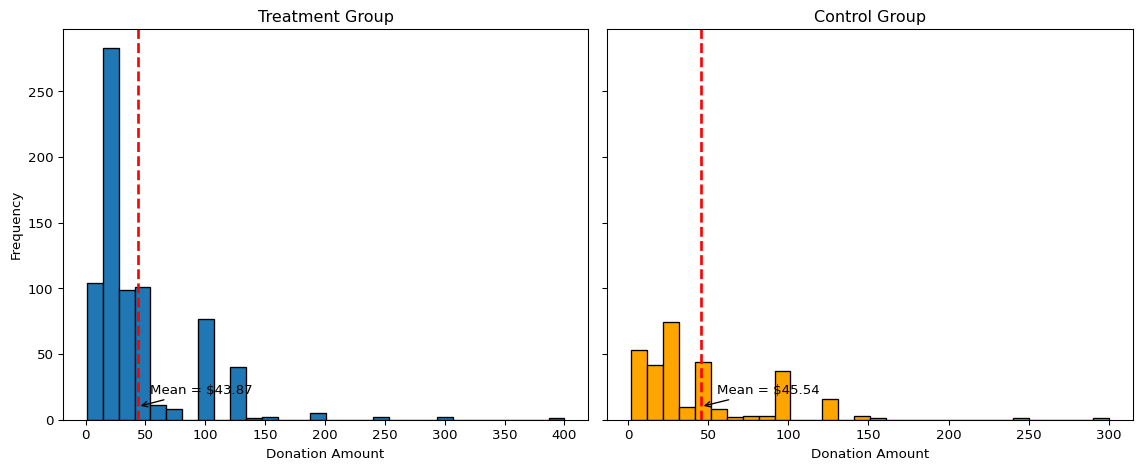
The histograms show the distribution of donation amounts among individuals who gave, separated by treatment group. Both distributions are right-skewed, with most donations concentrated at lower amounts. The red dashed lines mark the mean donation in each group: $43.87 for treatment and $45.54 for control. The similarity in means visually confirms earlier statistical results, indicating that while the presence of a match may influence whether someone donates, it does not significantly affect how much they give once they’ve decided to contribute.

Simulation Experiment

As a reminder of how the t-statistic “works,” in this section I use simulation to demonstrate the Law of Large Numbers and the Central Limit Theorem.

Suppose the true distribution of respondents who do not get a charitable donation match is Bernoulli with probability p=0.018 that a donation is made.

Further suppose that the true distribution of respondents who do get a charitable donation match of any size is Bernoulli with probability p=0.022 that a donation is made.

Law of Large Numbers

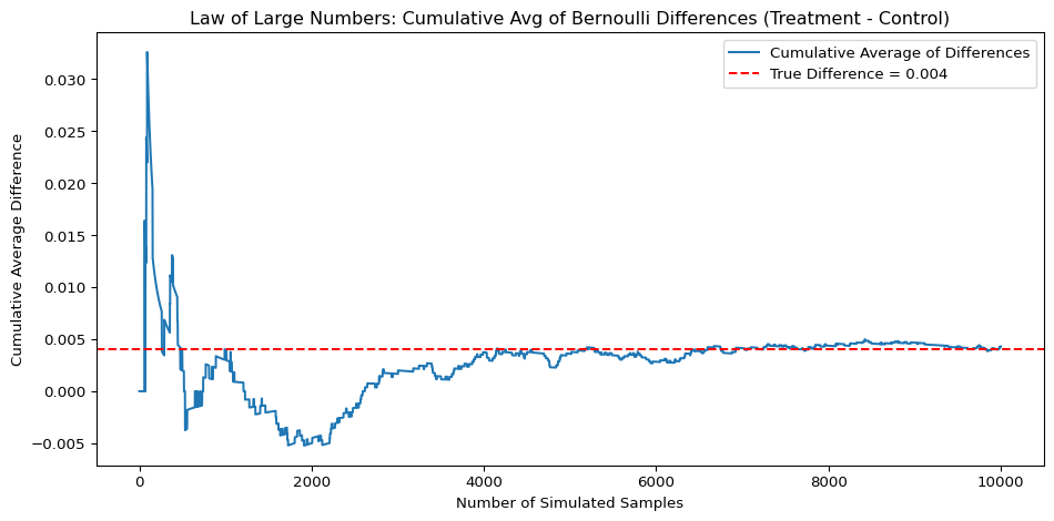
np.random.seed(42)

# Control group: Bernoulli(p=0.018), 100,000 draws
control_sim = np.random.binomial(n=1, p=0.018, size=100000)

# Treatment group: Bernoulli(p=0.022), 10,000 draws
treatment_sim = np.random.binomial(n=1, p=0.022, size=10000)

# diff_vector = treatment_sim - np.random.choice(control_sim, size=10000)
diff_vector = treatment_sim - control_sim[:10000]

cumulative_avg = np.cumsum(diff_vector) / np.arange(1, len(diff_vector) + 1)

true_diff = 0.022 - 0.018

plt.figure(figsize=(10, 5))
plt.plot(cumulative_avg, label='Cumulative Average of Differences')
plt.axhline(y=true_diff, color='red', linestyle='--', label=f'True Difference = {true_diff:.3f}')
plt.title('Law of Large Numbers: Cumulative Avg of Bernoulli Differences (Treatment - Control)')
plt.xlabel('Number of Simulated Samples')
plt.ylabel('Cumulative Average Difference')
plt.legend()
plt.tight_layout()
plt.show()

This plot illustrates the Law of Large Numbers using simulated donation data. I calculated the cumulative average difference in donation rates between treatment (2.2 percent) and control (1.8 percent) groups across 10,000 simulated comparisons. The blue line shows how the average difference stabilizes, while the red dashed line marks the true difference (0.004). As more samples accumulate, the cumulative average converges to the true value, confirming that larger samples yield more reliable estimates.

Central Limit Theorem

sample_sizes = [50, 200, 500, 1000]
simulations = 1000
p_control = 0.018
p_treatment = 0.022

diff_distributions = {}

np.random.seed(42)

for n in sample_sizes:
    diffs = []
    for _ in range(simulations):
        control_draw = np.random.binomial(1, p_control, n)
        treatment_draw = np.random.binomial(1, p_treatment, n)
        mean_diff = treatment_draw.mean() - control_draw.mean()
        diffs.append(mean_diff)
    diff_distributions[n] = diffs

fig, axes = plt.subplots(2, 2, figsize=(12, 8))
axes = axes.flatten()

for i, n in enumerate(sample_sizes):
    axes[i].hist(diff_distributions[n], bins=30, edgecolor='black', alpha=0.7)
    axes[i].axvline(0, color='black', linestyle='--', label='Zero')
    axes[i].set_title(f"Sample Size = {n}")
    axes[i].set_xlabel("Mean Difference (Treatment - Control)")
    axes[i].axvline(p_treatment - p_control, color='red', linestyle='--', label='True Difference')
    axes[i].set_ylabel("Frequency")
    axes[i].legend()

plt.tight_layout()
plt.show()

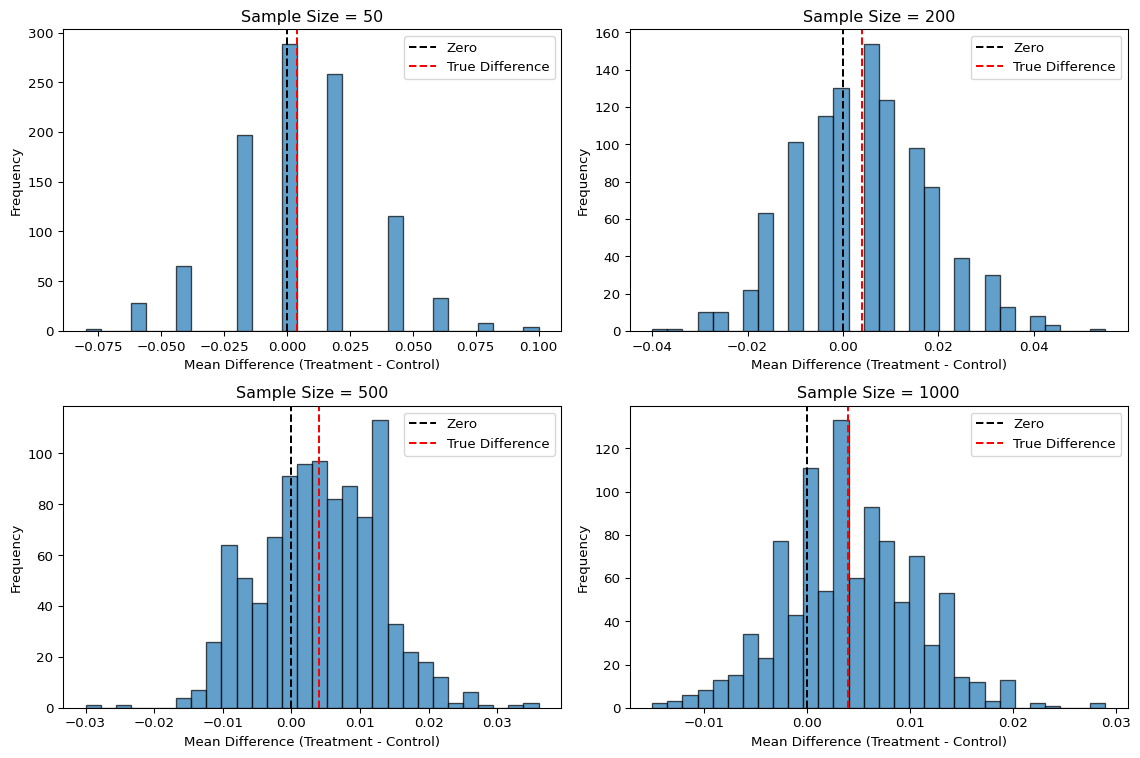
These histograms show the distribution of average differences in donation rates between treatment and control groups across 1,000 simulations at sample sizes of 50, 200, 500, and 1000. At smaller sizes, the distributions are wide and zero (red) is near the center, reflecting high uncertainty. As the sample size grows, the distributions narrow and more centered around the true difference (black) and zero (red) moves toward the tail, making it less likely. This demonstrates the Central Limit Theorem and shows that larger samples improve our ability to detect small treatment effects.